Soil Heat‑Flux Estimation & Validation
This notebook demonstrates how to derive surface ground‑heat flux (G₀) from a SoilVUE profile using the helper functions included in the project repository, and then compares the derived values with the in‑situ heat‑flux‑plate measurements (“G”) available in the eddy‑covariance flux file.
Data files used:
File |
Contents |
Native resolution |
|---|---|---|
|
SoilVUE profile statistics (T, VWC, κ etc.) |
Site‑logger native (≈ 5–10 min) |
|
30‑min AmeriFlux‑format flux file (includes G) |
30 min |
The analysis proceeds as follows:
Load & tidy the two datasets.
Estimate ground‑heat flux from the SoilVUE temperatures and soil‑moisture–dependent conductivity using
soil_heat.compute_heat_flux_conduction.Merge the estimated series with the measured 30‑min “G” record.
Evaluate performance using RMSE & NME (functions in
gao_et_al.py) and quick visualisations.
Note – The SoilVUE statistics file shipped with this example has a single timestamp header (
2024‑07‑11). Rows are therefore back‑filled with that value and treated as measurements for 11 July 2024. If your logger exports full timestamps, simply remove the forward‑fill block below.
Import relevant libraries
[ ]:
[2]:
import pandas as pd
import numpy as np
import matplotlib.pyplot as plt
from pathlib import Path
import sys
import micromet
# Project helper modules (all live in /mnt/data after upload)
sys.path.append('../../src')
import soil_heat                     # gradient & calorimetric methods
#import gao_et_al as gao              # RMSE & NME helpers
[3]:
station_path = Path("G:/Shared drives/UGS_Flux/Data_Downloads/Dugout_Ranch/")
Load SoilVUE Data
[4]:
dfs = {}

for file in station_path.rglob("*21031_Statistics_AmeriFlux*.dat"):
    fileno = file.stem.split("_")[-1].replace("AmeriFlux", "")
    dfs[fileno] = pd.read_csv(file, na_values=['NAN'], engine='python',)
df_sv = pd.concat(dfs,ignore_index=True).iloc[50:,:57]

# Back‑fill the one timestamp so that every row carries a datetime label
df_sv['TIMESTAMP_START'] = df_sv['TIMESTAMP_START'].ffill()

# Parse to pandas datetime (format YYYYMMDDhhmm)
df_sv['datetime'] = pd.to_datetime(df_sv['TIMESTAMP_START'], format='%Y%m%d%H%M')

# For this demo we keep only the channels needed for the gradient method
df_sv = df_sv.astype({'T_1_1_1': float,
                      'T_1_2_1': float,
                        'T_1_3_1': float,
                        'T_1_4_1': float,
                        'T_1_5_1': float,
                        'T_1_6_1': float,
                        'T_1_7_1': float,
                      'VWC_1_1_1': float,
                      'VWC_1_2_1': float,
                        'VWC_1_3_1': float,
                        'VWC_1_4_1': float,
                        'VWC_1_5_1': float,
                        'VWC_1_6_1': float,
                        'VWC_1_7_1': float,
                        'T_CANOPY': float,
                        'NETRAD': float,
                        'SW_IN': float,
                        'SW_OUT': float,
                        'LW_IN': float,
                        'LW_OUT': float,
                      })
df_sv = df_sv.set_index('datetime').sort_index().drop_duplicates()
df_sv = df_sv.loc[pd.to_datetime('2023-07-01'):]

#df_sv['datetime'] = pd.date_range(start='2024-07-11 05:30', periods=589, freq='30min')
# Package expects the DataFrame columns to be named explicitly
df_grad =df_sv.rename(columns={
    'T_CANOPY':'T00cm',
    'T_1_1_1':'T05cm',
    'T_1_2_1':'T10cm',
    'T_1_3_1':'T20cm',
    'T_1_4_1':'T30cm',
    'T_1_5_1':'T40cm',
    'T_1_6_1':'T50cm',
    'T_1_7_1':'T60cm',
    'VWC_1_1_1':'VWC05cm',
    'VWC_1_2_1':'VWC10cm',
    'VWC_1_3_1':'VWC20cm',
    'VWC_1_4_1':'VWC30cm',
    'VWC_1_5_1':'VWC40cm',
    'VWC_1_6_1':'VWC50cm',
    'VWC_1_7_1':'VWC60cm',
})
[5]:
df_grad
[5]:
| TIMESTAMP_START | TIMESTAMP_END | ALB | NETRAD | SW_IN | SW_OUT | LW_IN | LW_OUT | T00cm | T_SI111_body | ... | WS | WD | LWmV_1_1_1 | LWMDry_1_1_1 | LWMCon_1_1_1 | LWMWet_1_1_1 | LWmV_1_1_2 | LWMDry_1_1_2 | LWMCon_1_1_2 | LWMWet_1_1_2 | |
|---|---|---|---|---|---|---|---|---|---|---|---|---|---|---|---|---|---|---|---|---|---|
| datetime | |||||||||||||||||||||
| 2023-07-20 09:41:00 | 2.023072e+11 | 2.023072e+11 | 28.26583 | 318.8813 | 637.4134 | 180.1522 | 357.5272 | 495.9071 | 32.17941 | 28.71401 | ... | 2.701577 | 306.6066 | 257.1425 | 62.5 | 0.0 | 0.0 | 255.5927 | 62.5 | 0.0 | 0.0 |
| 2023-07-20 10:00:00 | 2.023072e+11 | 2.023072e+11 | 28.15890 | 356.0205 | 707.7589 | 199.2483 | 358.8571 | 511.3472 | 34.38037 | 29.93085 | ... | 2.064533 | 281.3860 | 256.7885 | 100.0 | 0.0 | 0.0 | 255.1927 | 100.0 | 0.0 | 0.0 |
| 2023-07-20 10:30:00 | 2.023072e+11 | 2.023072e+11 | 27.51952 | 412.0310 | 787.1783 | 216.5737 | 362.4536 | 521.0272 | 35.60567 | 30.57986 | ... | 3.209229 | 283.3472 | 256.8130 | 100.0 | 0.0 | 0.0 | 255.2341 | 100.0 | 0.0 | 0.0 |
| 2023-07-20 11:00:00 | 2.023072e+11 | 2.023072e+11 | 27.00862 | 456.5611 | 858.3252 | 231.7979 | 364.8067 | 534.7730 | 37.48657 | 30.97627 | ... | 2.742912 | 299.0038 | 256.7047 | 100.0 | 0.0 | 0.0 | 255.3200 | 100.0 | 0.0 | 0.0 |
| 2023-07-20 11:30:00 | 2.023072e+11 | 2.023072e+11 | 26.51160 | 498.9389 | 917.5994 | 243.2511 | 371.8264 | 547.2357 | 39.28394 | 32.05534 | ... | 2.307465 | 340.5045 | 256.3628 | 100.0 | 0.0 | 0.0 | 255.1371 | 100.0 | 0.0 | 0.0 |
| ... | ... | ... | ... | ... | ... | ... | ... | ... | ... | ... | ... | ... | ... | ... | ... | ... | ... | ... | ... | ... | ... |
| 2025-05-13 09:00:00 | 2.025051e+11 | 2.025051e+11 | 23.49375 | 446.7189 | 761.8327 | 178.9415 | 289.9461 | 426.1184 | 19.63299 | 21.44107 | ... | 5.782328 | 148.2818 | 258.6791 | 100.0 | 0.0 | 0.0 | 258.3070 | 100.0 | 0.0 | 0.0 |
| 2025-05-13 09:30:00 | 2.025051e+11 | 2.025051e+11 | 22.89209 | 509.1336 | 835.5638 | 191.2458 | 294.1239 | 429.3082 | 20.33200 | 21.40081 | ... | 6.696503 | 144.6211 | 258.6787 | 100.0 | 0.0 | 0.0 | 258.4439 | 100.0 | 0.0 | 0.0 |
| 2025-05-13 10:00:00 | 2.025051e+11 | 2.025051e+11 | 22.35525 | 563.4611 | 901.9198 | 201.5875 | 297.2929 | 434.1642 | 21.22629 | 21.79152 | ... | 6.626107 | 142.0318 | 258.4643 | 100.0 | 0.0 | 0.0 | 258.7210 | 100.0 | 0.0 | 0.0 |
| 2025-05-13 10:30:00 | 2.025051e+11 | 2.025051e+11 | 21.78752 | 605.3776 | 951.9034 | 207.3797 | 300.8767 | 440.0228 | 22.18126 | 22.40828 | ... | 5.935644 | 149.8918 | 258.2034 | 100.0 | 0.0 | 0.0 | 258.9913 | 100.0 | 0.0 | 0.0 |
| 2025-05-13 11:00:00 | 2.025051e+11 | 2.025051e+11 | 21.38042 | 637.4340 | 990.0894 | 211.6744 | 301.4280 | 442.4090 | 22.66282 | 22.57568 | ... | 6.051284 | 149.1903 | 258.0860 | 100.0 | 0.0 | 0.0 | 258.5698 | 100.0 | 0.0 | 0.0 |
28638 rows × 57 columns
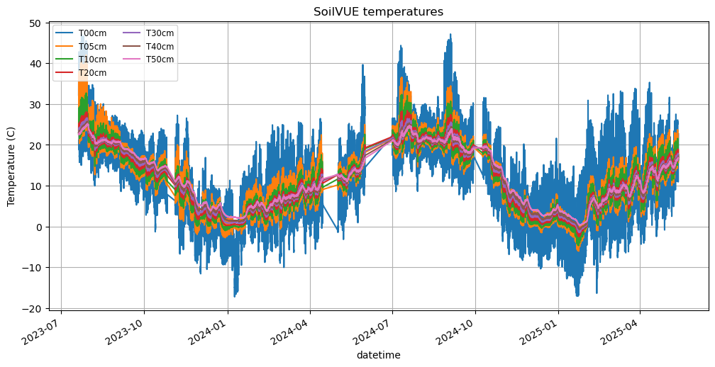
Plot SoilVUE data
Include data from the SI-111, which is technically measuring Temperature of the canopy top, but is T0cm for the timeframe being examined.
[6]:
df_grad[['T00cm','T05cm', 'T10cm', 'T20cm', 'T30cm','T40cm','T50cm']].plot(title='SoilVUE temperatures', ylabel='Temperature (C)', figsize=(12, 6))
plt.legend(loc='upper left', fontsize='small', ncol=2)
plt.grid(True)
plt.savefig('soilvue_temperatures.png', dpi=300, bbox_inches='tight')
Initial Estimate of G0
[7]:
# ---------- Parameters ------------------------------------------------------
DEPTH_TOP  = 0.05   # m  (sensor 1)
DEPTH_LOW  = 0.10   # m  (sensor 2)

# ---- Call helper – returns a pd.Series (W m‑2, positive downward)
G0_est = soil_heat.compute_heat_flux_conduction(
    df_grad,
    depth1=DEPTH_TOP,
    depth2=DEPTH_LOW,
    col_T1='T05cm',
    col_T2='T10cm',
    col_theta1='VWC05cm',
    col_theta2='VWC10cm',
    porosity = 0.5,
    k_dry = 0.45,
    k_sat = 2
)

G0_est_2 = soil_heat.compute_heat_flux_calorimetric(df_grad,depth_levels=[0.05,0.1,0.2,0.3],T_cols=['T05cm', 'T10cm','T20cm','T30cm'],theta_cols=['VWC05cm', 'VWC10cm', 'VWC20cm', 'VWC30cm'], )
Calculate amplitude and lag of data
[8]:
amp_values = pd.concat([soil_heat.diurnal_amplitude(df_grad['T00cm']),
                        soil_heat.diurnal_amplitude(df_grad['T05cm']),
                        soil_heat.diurnal_amplitude(df_grad['T10cm']),
                        soil_heat.diurnal_amplitude(df_grad['T20cm']),
                        soil_heat.diurnal_amplitude(df_grad['T30cm']),
],axis=1).round(2).rename(columns={
    'T00cm':'T00cm_amp',
    'T05cm':'T05cm_amp',
    'T10cm':'T10cm_amp',
    'T20cm':'T20cm_amp',
    'T30cm':'T30cm_amp',
})

amp_values
[8]:
| T00cm_amp | T05cm_amp | T10cm_amp | T20cm_amp | T30cm_amp | |
|---|---|---|---|---|---|
| datetime | |||||
| 2023-07-20 | 24.01 | 14.31 | 6.49 | 2.49 | 1.28 |
| 2023-07-21 | 26.98 | 17.68 | 7.84 | 3.09 | 1.55 |
| 2023-07-22 | 27.36 | 19.15 | 9.20 | 3.77 | 1.97 |
| 2023-07-23 | 32.12 | 19.26 | 9.13 | 3.58 | 1.84 |
| 2023-07-24 | 26.79 | 16.73 | 8.07 | 2.93 | 1.42 |
| ... | ... | ... | ... | ... | ... |
| 2025-05-09 | 16.61 | 11.11 | 7.85 | 3.66 | 2.21 |
| 2025-05-10 | 18.50 | 9.19 | 6.55 | 3.04 | 1.83 |
| 2025-05-11 | 14.63 | 7.97 | 5.55 | 2.48 | 1.39 |
| 2025-05-12 | 14.91 | 9.42 | 6.57 | 2.96 | 1.73 |
| 2025-05-13 | 11.74 | 3.12 | 1.94 | 1.52 | 1.00 |
664 rows × 5 columns
[10]:
diff_00_10 = soil_heat.thermal_diffusivity_amplitude(amp_values['T00cm_amp'], amp_values['T10cm_amp'],z1=0.00,z2=0.10)#.median()#.plot(label='T00cm to T10cm')
diff_00_05 = soil_heat.thermal_diffusivity_amplitude(amp_values['T00cm_amp'], amp_values['T05cm_amp'],z1=0.00,z2=0.05)#.median()#.plot(label='T00cm to T05cm')
diff_05_10 = soil_heat.thermal_diffusivity_amplitude(amp_values['T05cm_amp'], amp_values['T10cm_amp'],z1=0.05,z2=0.10)#.median()#.plot(label='T05cm to T10cm')
diff = pd.concat([diff_00_10, diff_00_05, diff_05_10], axis=1)#.plot(title='Thermal diffusivity (amplitude method)', ylabel='m² s⁻¹')
diff['median'] = diff.median(axis=1)
#soil_heat.thermal_diffusivity_amplitude(amp_values['T05cm_amp'], amp_values['T20cm_amp'],z1=0.00,z2=0.20).plot(label='T05cm to T20cm')
#soil_heat.thermal_diffusivity_amplitude(amp_values['T05cm_amp'], amp_values['T30cm_amp'],z1=0.05,z2=0.30).plot()
#soil_heat.thermal_diffusivity_amplitude(amp_values['T10cm_amp'], amp_values['T20cm_amp'],z1=0.10,z2=0.20).plot()
print(f"Thermal diffusivity (T00cm to T10cm): {diff_00_10.median():.7f} m² s⁻¹")
print(f"Thermal diffusivity (T00cm to T05cm): {diff_00_05.median():.7f} m² s⁻¹")
print(f"Thermal diffusivity (T05cm to T10cm): {diff_05_10.median():.7f} m² s⁻¹")
print(f"Mean Thermal diffusivity (T00cm to T10cm): {np.mean([diff_00_10.median(),diff_00_05.median(),diff_05_10.median()]):.7f} m² s⁻¹")
Thermal diffusivity (T00cm to T10cm): 0.0000002 m² s⁻¹
Thermal diffusivity (T00cm to T05cm): 0.0000001 m² s⁻¹
Thermal diffusivity (T05cm to T10cm): 0.0000004 m² s⁻¹
Mean Thermal diffusivity (T00cm to T10cm): 0.0000002 m² s⁻¹
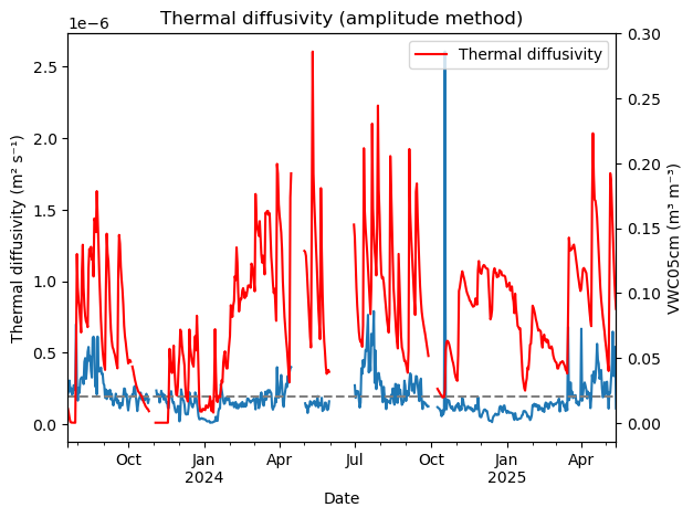
[11]:
diff['median'].plot(title='Thermal diffusivity (amplitude method)', ylabel='Thermal diffusivity (m² s⁻¹)')
plt.axhline(y=diff['median'].mean(), color='grey', linestyle='--', label='Mean diffusivity')
plt.xlabel('Date')
plt.twinx()
df_grad['VWC05cm'].resample('D').mean().plot(color='red')
plt.ylabel('VWC05cm (m³ m⁻³)')
plt.legend(['Thermal diffusivity', 'VWC05cm'])
[11]:
<matplotlib.legend.Legend at 0x25ab97cc550>
[12]:
import numpy as np
import pandas as pd
from soil_heat import (diurnal_amplitude, thermal_diffusivity_amplitude)

import numpy as np
import pandas as pd
from soil_heat import diurnal_amplitude, thermal_diffusivity_amplitude

def estimate_rhoc_dry(
    alpha: pd.Series,
    theta: pd.Series,
    porosity: float = 0.40,
    k_dry: float = 0.25,
    k_sat: float = 1.50,
    rhoc_w: float = 4.18e6,
    dry_quantile: float = 0.10,
) -> float:
    """Return volumetric heat capacity of *dry* soil (J m⁻³ K⁻¹)."""

    # keep only days where both alpha & theta are available
    theta, alpha = theta.align(alpha, join='inner')          # ⬅ key line

    frac_sat = np.clip(theta / porosity, 0.0, 1.0)
    lam = k_dry + (k_sat - k_dry) * frac_sat                 # W m⁻¹ K⁻¹

    # --- 3. Heat capacity & dry-soil estimate ------------------
    Cv = lam / alpha                                         # J m⁻³ K⁻¹
    rhoc_dry = (Cv - theta * rhoc_w) / (1.0 - theta)

    dry_days = theta <= theta.quantile(dry_quantile)
    return float(rhoc_dry.loc[dry_days].median())
[13]:
alpha_daily = diff['median']
theta_daily = df_grad['VWC05cm'].resample('D').mean()

estimate_rhoc_dry(alpha_daily, theta_daily, porosity=0.40, k_dry=0.25, k_sat=1.50, rhoc_w=4.18e6, dry_quantile=0.10)*1e-6
[13]:
1.6819569524012492
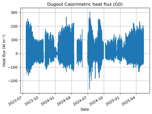
[18]:
G0 = soil_heat.compute_heat_flux_calorimetric(
    df_grad,
    depth_levels = [0.05, 0.10, 0.20, 0.30],
    T_cols = ['T05cm', 'T10cm', 'T20cm', 'T30cm'],
    theta_cols = ['VWC05cm', 'VWC10cm', 'VWC20cm', 'VWC30cm'],
    C_dry = 1.72e6,
    C_w = 4.2e6,)
G0a = np.where(G0<-500,np.nan,G0)
G0a = np.where(G0a>500,np.nan,G0a)
G0 = pd.Series(G0a, index=df_grad.index, name='G0_calorimetric')
G0.plot()
plt.title('Dugout Calorimetric heat flux (G0)')
plt.xlabel('Date')
plt.ylabel('Heat flux (W m⁻²)')
plt.grid(True)
[ ]:
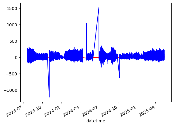
[78]:
G0_est.plot(label='G0_est_grad', color='red')
G0_est_2.plot(label='G0_est_calorimetric', color='blue')
[78]:
<Axes: xlabel='datetime'>
[32]:
eddy_station_path = Path("G:/Shared drives/UGS_Flux/Data_Downloads/Dugout_Ranch/Eddy")

dfs_edd = {}
# ---------- SoilVUE data ----------------------------------------------------
for file in eddy_station_path.glob("*Flux_AmeriFluxFormat*.dat"):
    fileno = file.stem.split("_")[-1].replace("AmeriFlux", "")
    #print(file.stem)
    dfs_edd[fileno] = pd.read_csv(file, na_values=['NAN'], engine='python',)
[ ]:
met_w_g = pd.concat([G0, G0_est, G0_est_2,df_grad], axis=1)
g = pd.concat([G0, G0_est, G0_est_2],axis=1)

eddy = pd.concat(dfs_edd, ignore_index=True)
eddy.drop(columns=['TIMESTAMP', 'RECORD'], inplace=True, errors='ignore')
eddy['datetime'] = pd.to_datetime(eddy['TIMESTAMP_START'], format='%Y%m%d%H%M')
eddy = eddy.set_index('datetime').sort_index().drop_duplicates()
met_n_eddy_g = pd.merge(eddy, met_w_g, left_index=True, right_index=True, how='outer', suffixes=('_eddy',''))
[105]:
for col in met_n_eddy_g.columns:
    if "NET" in col:
        print(col)
NETRAD_eddy
NETRAD
[106]:
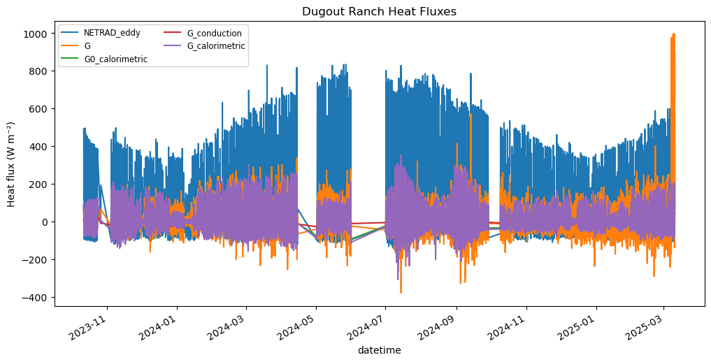
g_vals = met_n_eddy_g[['NETRAD_eddy','G','G0_calorimetric','G_conduction','G_calorimetric']].dropna()
g_vals = g_vals[g_vals.abs()<1000].dropna()  # Filter out extreme values
g_vals.plot(title='Dugout Ranch Heat Fluxes', ylabel='Heat flux (W m⁻²)', figsize=(12, 6))
plt.legend(loc='upper left', fontsize='small', ncol=2)
[106]:
<matplotlib.legend.Legend at 0x25adeb66fd0>
[107]:
#new_df = g
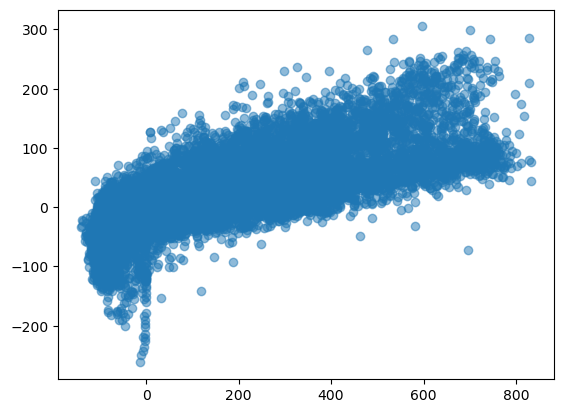
x = g_vals['NETRAD_eddy']
y = g_vals['G0_calorimetric']
plt.scatter(x, y, alpha=0.5)
import statsmodels.api as sm
X = sm.add_constant(x) # adds intercept term
model = sm.OLS(y, X).fit() # fit the model
print(model.summary())
                            OLS Regression Results
==============================================================================
Dep. Variable:        G0_calorimetric   R-squared:                       0.625
Model:                            OLS   Adj. R-squared:                  0.625
Method:                 Least Squares   F-statistic:                 3.647e+04
Date:                Sun, 15 Jun 2025   Prob (F-statistic):               0.00
Time:                        21:09:52   Log-Likelihood:            -1.0969e+05
No. Observations:               21909   AIC:                         2.194e+05
Df Residuals:                   21907   BIC:                         2.194e+05
Df Model:                           1
Covariance Type:            nonrobust
===============================================================================
                  coef    std err          t      P>|t|      [0.025      0.975]
-------------------------------------------------------------------------------
const         -15.8099      0.258    -61.317      0.000     -16.315     -15.305
NETRAD_eddy     0.2201      0.001    190.979      0.000       0.218       0.222
==============================================================================
Omnibus:                     1191.533   Durbin-Watson:                   0.252
Prob(Omnibus):                  0.000   Jarque-Bera (JB):             3759.978
Skew:                           0.231   Prob(JB):                         0.00
Kurtosis:                       4.976   Cond. No.                         236.
==============================================================================

Notes:
[1] Standard Errors assume that the covariance matrix of the errors is correctly specified.
[ ]:
ebal_g0 = met_n_eddy_g[['G0_calorimetric','NETRAD_eddy','LE','H','G','NETRAD']].dropna()
ebal_g0_daily = ebal_g0.resample('D').sum(min_count=48).dropna()
for col in ebal_g0_daily.columns:
if col not in ['NETRAD_eddy','NETRAD']:
ebal_g0_daily[col] = np.where(ebal_g0_daily[col].abs() > ebal_g0_daily['NETRAD_eddy'].abs(), np.nan, ebal_g0_daily[col])
ebal_g0_daily = ebal_g0_daily.dropna()
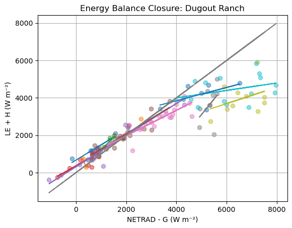
x = ebal_g0_daily['NETRAD_eddy'] - ebal_g0_daily['G0_calorimetric']
y = ebal_g0_daily['LE'] + ebal_g0_daily['H']
plt.scatter(x, y, alpha=0.5)
plt.xlabel('NETRAD - G (W m⁻²)')
plt.ylabel('LE + H (W m⁻²)')
X = sm.add_constant(x) # adds intercept term
model = sm.OLS(y, X).fit() # fit the model
print(model.summary())
plt.title('Energy Balance Closure: Dugout Ranch')
plt.grid(True)
plt.plot(x,model.predict(X), color='red', label='OLS Fit')
plt.plot(x, x, color='green', linestyle='--', label='1:1 Line')
[109]:
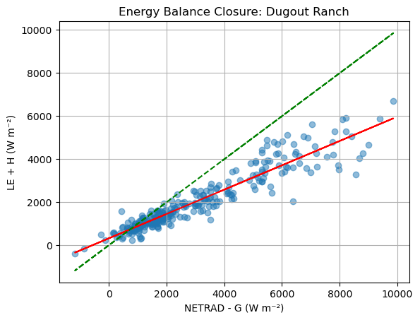
ebal_g0 = met_n_eddy_g[['G0_calorimetric','NETRAD_eddy','LE','H','G']].dropna()

ebal_g0_daily = ebal_g0.resample('D').sum(min_count=48).dropna()
for col in ebal_g0_daily.columns:
    if col != 'NETRAD_eddy':
        ebal_g0_daily[col] = np.where(ebal_g0_daily[col].abs() > ebal_g0_daily['NETRAD_eddy'].abs(), np.nan, ebal_g0_daily[col])
ebal_g0_daily = ebal_g0_daily.dropna()

x = ebal_g0_daily['NETRAD_eddy'] - ebal_g0_daily['G0_calorimetric']
y = ebal_g0_daily['LE'] + ebal_g0_daily['H']
plt.scatter(x, y, alpha=0.5)
plt.xlabel('NETRAD - G (W m⁻²)')
plt.ylabel('LE + H (W m⁻²)')
X = sm.add_constant(x)      # adds intercept term
model = sm.OLS(y, X).fit()  # fit the model
print(model.summary())
plt.title('Energy Balance Closure: Dugout Ranch')
plt.grid(True)

plt.plot(x,model.predict(X), color='red', label='OLS Fit')
plt.plot(x, x, color='green', linestyle='--', label='1:1 Line')
                            OLS Regression Results
==============================================================================
Dep. Variable:                      y   R-squared:                       0.887
Model:                            OLS   Adj. R-squared:                  0.886
Method:                 Least Squares   F-statistic:                     2151.
Date:                Sun, 15 Jun 2025   Prob (F-statistic):          4.97e-132
Time:                        21:10:36   Log-Likelihood:                -2090.7
No. Observations:                 277   AIC:                             4185.
Df Residuals:                     275   BIC:                             4193.
Df Model:                           1
Covariance Type:            nonrobust
==============================================================================
                 coef    std err          t      P>|t|      [0.025      0.975]
------------------------------------------------------------------------------
const        323.2827     46.499      6.952      0.000     231.744     414.822
0              0.5654      0.012     46.378      0.000       0.541       0.589
==============================================================================
Omnibus:                       21.781   Durbin-Watson:                   1.000
Prob(Omnibus):                  0.000   Jarque-Bera (JB):               76.449
Skew:                          -0.115   Prob(JB):                     2.51e-17
Kurtosis:                       5.563   Cond. No.                     6.41e+03
==============================================================================

Notes:
[1] Standard Errors assume that the covariance matrix of the errors is correctly specified.
[2] The condition number is large, 6.41e+03. This might indicate that there are
strong multicollinearity or other numerical problems.
[109]:
[<matplotlib.lines.Line2D at 0x25adf442490>]
[110]:
import scipy
for year in range(2023, 2025):
    for month in ebal_g0_daily.index.month.unique():
        df = ebal_g0_daily[(ebal_g0_daily.index.month == month)&(ebal_g0_daily.index.year == year)].dropna()
        if df.empty:
            continue
        else:
            x = df['NETRAD_eddy'] - df['G']
            y = df['LE'] + df['H']
            slope, intercept, r, p, se = scipy.stats.linregress(x, y)

            plt.scatter(x, y, alpha=0.5, label=f'Month {month}')
            plt.xlabel('NETRAD - G (W m⁻²)')
            plt.ylabel('LE + H (W m⁻²)')
            print(f"r-squared for {year}-{month}: {r*r:.3f}")

            print(f"Slope for {year}-{month}: {slope:.3f}")
            plt.title(f'Energy Balance Closure: Dugout Ranch')
            plt.grid(True)
            plt.plot(x, x*slope + intercept, label='OLS Fit')
            plt.plot(x, x, linestyle='--', label='1:1 Line',color='grey')
r-squared for 2023-11: 0.431
Slope for 2023-11: 0.597
r-squared for 2023-12: 0.431
Slope for 2023-12: 0.500
r-squared for 2024-11: 0.708
Slope for 2024-11: 0.793
r-squared for 2024-12: 0.308
Slope for 2024-12: 0.315
r-squared for 2024-1: 0.945
Slope for 2024-1: 0.500
r-squared for 2024-2: 0.784
Slope for 2024-2: 0.575
r-squared for 2024-3: 0.730
Slope for 2024-3: 0.483
r-squared for 2024-4: 0.549
Slope for 2024-4: 2.261
r-squared for 2024-7: 0.519
Slope for 2024-7: 0.753
r-squared for 2024-8: 0.099
Slope for 2024-8: 0.179
r-squared for 2024-9: 0.412
Slope for 2024-9: 0.668
r-squared for 2024-10: 0.369
Slope for 2024-10: 0.613
[101]:
import scipy
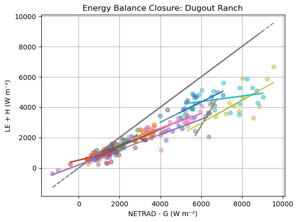
for year in range(2023, 2025):
for month in ebal_g0_daily.index.month.unique():
df = ebal_g0_daily[(ebal_g0_daily.index.month == month)&(ebal_g0_daily.index.year == year)].dropna()
if df.empty:
continue
else:
x = df['NETRAD'] - df['G0_calorimetric']
y = df['LE'] + df['H']
slope, intercept, r, p, se = scipy.stats.linregress(x, y)
plt.scatter(x, y, alpha=0.5, label=f'Month {month}')
plt.xlabel('NETRAD - G (W m⁻²)')
plt.ylabel('LE + H (W m⁻²)')
print(f"r-squared for {year}-{month}: {r*r:.3f}")
print(f"Slope for {year}-{month}: {slope:.3f}")
plt.title(f'Energy Balance Closure: Dugout Ranch')
plt.grid(True)
plt.plot(x, x*slope + intercept, label='OLS Fit')
plt.plot(x, x, linestyle='--', label='1:1 Line',color='grey')
r-squared for 2023-11: 0.850
Slope for 2023-11: 0.815
r-squared for 2023-12: 1.000
Slope for 2023-12: -4.294
r-squared for 2024-11: 0.869
Slope for 2024-11: 1.319
r-squared for 2024-12: 0.714
Slope for 2024-12: 0.757
r-squared for 2024-1: 0.910
Slope for 2024-1: 0.845
r-squared for 2024-2: 0.829
Slope for 2024-2: 0.820
r-squared for 2024-3: 0.817
Slope for 2024-3: 0.679
r-squared for 2024-4: 0.213
Slope for 2024-4: 1.657
r-squared for 2024-7: 0.140
Slope for 2024-7: 0.438
r-squared for 2024-8: 0.126
Slope for 2024-8: 0.199
r-squared for 2024-9: 0.339
Slope for 2024-9: 0.355
r-squared for 2024-10: 0.000
Slope for 2024-10: nan
c:\Users\paulinkenbrandt\.conda\envs\py313\Lib\site-packages\scipy\stats\_stats_py.py:10729: RuntimeWarning: invalid value encountered in scalar divide
  slope = ssxym / ssxm
c:\Users\paulinkenbrandt\.conda\envs\py313\Lib\site-packages\scipy\stats\_stats_py.py:10743: RuntimeWarning: invalid value encountered in sqrt
  t = r * np.sqrt(df / ((1.0 - r + TINY)*(1.0 + r + TINY)))
c:\Users\paulinkenbrandt\.conda\envs\py313\Lib\site-packages\scipy\stats\_stats_py.py:10749: RuntimeWarning: invalid value encountered in scalar divide
  slope_stderr = np.sqrt((1 - r**2) * ssym / ssxm / df)
[ ]:
# ---------- Eddy‑covariance flux data ---------------------------------------

flux_path_1 = station_path / "e20250513/21314_Flux_AmeriFluxFormat_22.dat"
flux_path_2 = station_path / "e20250513/21314_Flux_AmeriFluxFormat_23.dat"

df_flux_1 = pd.read_csv(flux_path_1, na_values=['NAN'])
df_flux_2 = pd.read_csv(flux_path_2, na_values=['NAN'])
df_flux = pd.concat([df_flux_1, df_flux_2], ignore_index=True)
# Parse timestamp and keep only ground‑heat flux variable ‘G’
df_flux['datetime'] = pd.to_datetime(df_flux['TIMESTAMP_START'].astype(str),
                                     format='%Y%m%d%H%M')

df_flux = df_flux[['datetime', 'G']].dropna(subset=['G']).astype({'G': float})

# Sub‑set to 11 July 2024 (matches the SoilVUE example file)
#mask_0711 = df_flux['datetime'].dt.strftime('%Y%m%d') == '20240711'
#df_flux_0711 = df_flux.loc[mask_0711].set_index('datetime')
#df_flux_0711.head()
df_flux
| datetime | G | |
|---|---|---|
| 0 | 2025-03-27 23:30:00 | -21.953250 |
| 1 | 2025-03-28 00:00:00 | 8.787329 |
| 2 | 2025-03-28 00:30:00 | -7.845843 |
| 3 | 2025-03-28 01:00:00 | 11.065370 |
| 4 | 2025-03-28 01:30:00 | -7.604448 |
| ... | ... | ... |
| 2227 | 2025-05-13 09:00:00 | -36.622820 |
| 2228 | 2025-05-13 09:30:00 | -21.398640 |
| 2229 | 2025-05-13 10:00:00 | -1.253632 |
| 2230 | 2025-05-13 10:30:00 | 21.987450 |
| 2231 | 2025-05-13 11:00:00 | 7.689254 |
2232 rows × 2 columns
[42]:
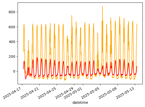
df_grad['NETRAD'].plot(label='NETRAD', color='orange')
G0.plot(label='G0_est_grad', color='red')
[42]:
<Axes: xlabel='datetime'>
[ ]:
G0
datetime
2025-04-17 08:06:00          NaN
2025-04-17 08:30:00    30.251806
2025-04-17 09:00:00    46.027718
2025-04-17 09:30:00    66.398487
2025-04-17 10:00:00    84.717237
                         ...
2025-05-13 09:00:00    10.241025
2025-05-13 09:30:00    35.440317
2025-05-13 10:00:00    43.507711
2025-05-13 10:30:00    56.521603
2025-05-13 11:00:00    67.905579
Name: G_calorimetric, Length: 1255, dtype: float64
[43]:
df_NETRAD_G0 = pd.concat([df_grad['NETRAD'], G0], axis=1).dropna()

x = df_NETRAD_G0['NETRAD']
y = df_NETRAD_G0['G_calorimetric']

import statsmodels.api as sm

X = sm.add_constant(x)      # adds intercept term
model = sm.OLS(y, X).fit()  # fit the model
print(model.summary())
                            OLS Regression Results
==============================================================================
Dep. Variable:         G_calorimetric   R-squared:                       0.856
Model:                            OLS   Adj. R-squared:                  0.856
Method:                 Least Squares   F-statistic:                     7441.
Date:                Sun, 15 Jun 2025   Prob (F-statistic):               0.00
Time:                        08:23:29   Log-Likelihood:                -5817.9
No. Observations:                1254   AIC:                         1.164e+04
Df Residuals:                    1252   BIC:                         1.165e+04
Df Model:                           1
Covariance Type:            nonrobust
==============================================================================
                 coef    std err          t      P>|t|      [0.025      0.975]
------------------------------------------------------------------------------
const        -29.8550      0.796    -37.527      0.000     -31.416     -28.294
NETRAD         0.2374      0.003     86.259      0.000       0.232       0.243
==============================================================================
Omnibus:                       79.228   Durbin-Watson:                   0.524
Prob(Omnibus):                  0.000   Jarque-Bera (JB):              308.820
Skew:                           0.137   Prob(JB):                     8.72e-68
Kurtosis:                       5.416   Cond. No.                         325.
==============================================================================

Notes:
[1] Standard Errors assume that the covariance matrix of the errors is correctly specified.
[45]:
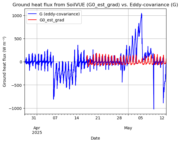
df_flux.plot(x='datetime', y='G', label='G (eddy‑covariance)', color='blue')
G0.plot(label='G0_est_grad', color='red',)
plt.xlabel('Date')
plt.ylabel('Ground heat flux (W m⁻²)')
plt.title('Ground heat flux from SoilVUE (G0_est_grad) vs. Eddy‑covariance (G)')
plt.legend()
plt.grid(True)
[ ]:
# Resample the high‑resolution SoilVUE estimates to 30‑min mean
G0_est_30min = G0_est.resample('30min').mean()

# Align indices (inner join)
df_cmp = pd.concat([G0_est_30min, df_flux_0711['G']], axis=1).dropna()
df_cmp.head()
| G_conduction | G | |
|---|---|---|
| datetime | ||
| 2024-07-11 05:30:00 | -26.632568 | -97.07862 |
| 2024-07-11 06:00:00 | -23.820008 | -42.72312 |
| 2024-07-11 06:30:00 | -19.676980 | -60.82810 |
| 2024-07-11 07:00:00 | -14.842567 | 13.72619 |
| 2024-07-11 07:30:00 | -6.595578 | 49.94262 |
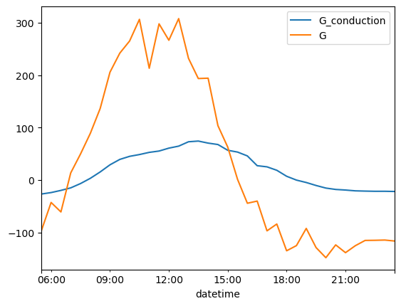
[ ]:
df_cmp.plot()
<Axes: xlabel='datetime'>
[ ]:
rmse_val = gao.rmse(df_cmp['G0_est_grad'].values, df_cmp['G'].values)
nme_val  = gao.nme(df_cmp['G0_est_grad'].values, df_cmp['G'].values)

print(f'RMSE  = {rmse_val:6.2f} W m⁻²')
print(f'NME   = {nme_val:6.2f} %')
[ ]:
# ---------- Time‑series overlay --------------------------------------------
plt.figure(figsize=(10, 4))
df_cmp['G0_est_grad'].plot(label='Estimated G₀ (gradient)', lw=1.2)
df_cmp['G'].plot(label='Measured G (plate)', lw=1.2)
plt.axhline(0, color='k', lw=0.4)
plt.ylabel('W m$^{-2}$')
plt.title('11 Jul 2024  •  30‑min surface ground‑heat flux')
plt.legend()
plt.tight_layout()
plt.show()

# ---------- Scatter plot ----------------------------------------------------
plt.figure(figsize=(4, 4))
plt.scatter(df_cmp['G'], df_cmp['G0_est_grad'], s=20)
plt.plot([-150, 150], [-150, 150], 'k--', lw=0.7)
plt.xlabel('Measured G (W m$^{-2}$)')
plt.ylabel('Estimated G₀ (W m$^{-2}$)')
plt.title('Gradient method performance')
plt.tight_layout()
plt.show()